Rohmer Damien
Arkadiusz Sitek
Grant T. Gullberg
Lawrence Berkeley National Laboratory
Report: LBNL-61064
Reconstruction and Visualization of Fiber and Laminar Structure in the Normal Human Heart.

Background — The human heart is composed of a helical network of muscle fibers. These fibers are organized to form sheets that are separated by cleavage surfaces. This complex structure of fibers and sheets is responsible for the orthotropic mechanical properties of cardiac muscle. The understanding of the configuration of the 3D fiber and sheet structure is important for modeling the mechanical and electrical properties of the heart and changes in this configuration may be of significant importance to understand the remodeling after myocardial infarction.
Methods — Anisotropic least square filtering followed by fiber and sheet tracking techniques were applied to Diffusion Tensor Magnetic Resonance Imaging (DTMRI) data of the excised human heart. The fiber configuration was visualized by using thin tubes to increase 3-dimensional visual perception of the complex structure. The sheet structures were reconstructed from the DTMRI data, obtaining surfaces that span the wall from the endo- to the epicardium. All visualizations were performed using the high-quality ray-tracing software POV-Ray.
Results — The fibers are shown to lie in sheets that have concave or convex transmural structure which correspond to histological studies published in the literature. The fiber angles varied depending on the position between the epi- and endocardium. The sheets had a complex structure that depended on the location within the myocardium. In the apex region the sheets had more curvature.
Conclusion — A high-quality visualization algorithm applied to demonstrate high quality DTMRI data is able to elicit the comprehension of the complex 3 dimensional structure of the fibers and sheets in the heart.
keywords: Cardiac Imaging, Diffusion Tensor MRI, Fiber Tracking, Laminar Architecture, Anisotropic filtering.

1 Introduction

DIFFUSION tensor magnetic resonance imaging (DTMRI) is a recently developed technique which enables the estimation of the diffusion tensor in biological samples. DTMRI is currently widely used in brain imaging to relate the connectivity network of the white matter axons to the diffusion data by estimating the principal direction of diffusion [1, 2]. In the current work fiber and laminar structure of the heart was determined from DTMRI data. A method for estimating the fiber and sheet geometry in the heart from DTMRI data is developed and a high quality visualization of the fiber and sheet structure inside the left ventricle of the human heart is demonstrated. The movement of the left ventricle is a mixture of contraction, extension and torsion [3]. This complex beating movement is due to a network of muscle fibers which wrap both ventricles [4, 5, 6]. The cardiac motion is created by contraction and extension of the cardiac fibers along which the diffusion is the largest (similar to the brain). However, in the cardiac muscle the fibers are arranged in sheet bundles. These sheets create a laminar structure that is responsible for the mechanical properties of the cardiac muscle [7, 8].

1.1 Structure of the heart

The geometry of the cardiac left ventricle can be approximated by a portion of an ellipsoid. The ellipsoid geometry is well described in the cylindrical coordinates (r,θ,z) (see Fig. 1). And its basis (e_r,e_θ,e_z) where bold letters are used for vectors. e _r refers to the radial component transverse to the wall, e _θ is the circumferential and e _z is the axial component from apex to base.

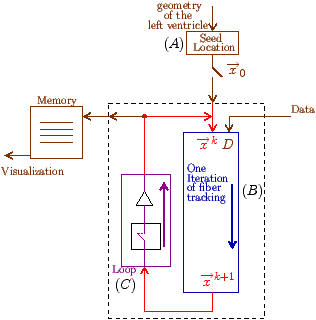
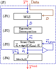
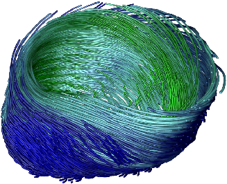
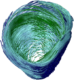
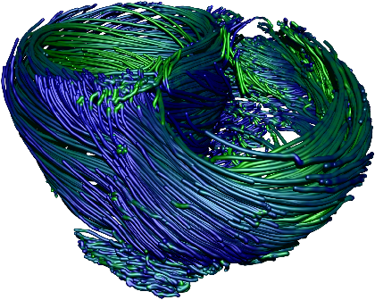
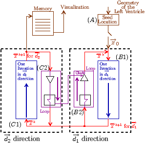
Fig. 1: [

Heart Anatomy]Heart Anatomy and cylindrical coordinate system that describes the cardiac geometry. The section represented is the posterior wall of the left and right ventricle. e _r is the radial component going across the wall, e _θ is the circumferential vector turning around the cylindrical geometry and e _z is the axial vector directed from the apex to the base. Each position of the myocardium is then specified by the three coordinates (r,θ,z).

1.1.1 Fiber Structure

The left ventricle is organized by a collection of 3 dimensional muscular fibers composed of myocytes (muscle cell) (see Fig. 2(a)). Each are 80 to 100 μ m in length and have a cylindrical shape with a radius of 5 to 10 μ m [9]. To enable the continuity of the electrical conduction along the fibers, consecutive cells are linked by gap (disc) junctions up to 8 μ m [10]. To preserve the tissue architecture especially during large deformations during contractile motion, cardiac fibers are embedded in an extracellular matrix, which consists of collagen and prevents muscle fiber slippage or rupture, protects from overstretching, and assists in the relengthening [11]. This extracellular collagen consists mainly of type I and III where type I corresponds to high tensile strength material and type III to highly deformable material [12]. The network linking adjacent fibers is called the endomysium (Fig. 2(a)) where the collagen of type III has the highest proportion (62%) compared to the collagen of type I. The collagen bundle is composed of fibrils with diameter ranging between 120 and 150 nm. Those are aligned primarily transverse to the direction of the muscle fiber [13]. The muscle fibers have a helical structure within the left ventricle. We will refer to α as the fiber angle: angle between e _θ and the direction of the fiber e _f (see Fig. 2(b) and Fig. 3). Histological studies and DTMRI measurements [14] have shown that the orientation of the fiber angle α varies continuously from +60^∘ to −60^∘ across the wall [6, 4]. Hence, the fibers turn clockwise from the apex to the base at the epicardium, have circular geometry in the midwall, and go counterclockwise close to the endocardium.

[] []

Fig. 2: [

Fiber and Sheet Anatomy]Figure (a) shows the geometry of the fiber and endomysial collagen in the heart. The long oval structures correspond to the fibers. Figure (b) shows the laminar structure with the cylindrical basis ( e _r, e _θ, e _z) and the sheet basis ( e _f, e _s, e _n).

1.1.2 Laminar Structure

Fibers in the heart form another three dimensional structure, due to the alignment of the fibers in sheets. Histological studies show that the fibers are grouped in a volume of three to four cells thick within a laminar structure oriented transversally to the heart-wall. The surface orientation of these sheets varies spatially showing a complex structure inside the heart [8]. The laminar structure can be roughly seen as twisted surfaces going across the wall and stacked from apex to base (see Fig. 2(b)). The sheets are physically separated by a coiled bundle of collagen fibers called perimysium [9]. These collagen fibrils are mainly oriented parallel to the long axis of the myocytes in the left ventricle [15]. This collagen consist mainly of type I (72%) (high tensile stength). The local geometry of the cleavage plane is characterized by the normal of the sheet at each position. We denote e _n this normal vector; and with the direction e _f of the fiber, we can define an orthonormal basis ( e _f, e _s, e _n) where e _s is perpendicular to the myocyte lying inside the sheet plane. We denote the angle between e_r and e_s the sheet angle β (see Fig. 2(b) and Fig. 3). Histology measurements have shown that this angle varies with the position across the wall (from +45^∘ to −80^∘) and the distribution changes from the apical region (roughly convex variation across the wall) to the basal region (concave variation) [8, 16].

1.1.3 Role of the fiber and laminar structure

The understanding of the laminar structure in the heart is of utmost importance for understanding the mechanical properties of the beating heart. It was postulated by Streeter et al. in 1969 that the fibers during cardiac contractions are subject to small homogeneous deformations in the entire left ventricle [5]. However, recent studies show that stress and strain have an orthotropic distribution in order to explain the change of the wall thickness between diastolic and systolic configuration of the heart [17, 18, 19]. Not only fiber but also the laminar structure is important to understand the complex motion of the myocardium and the orthotropic distribution of stress inside the heart along fiber and sheet directions [16, 7, 20, 21]. The link between laminar architecture and mechanics of the heart has been widely studied. Moreover, the study of the heart after myocardial infarction shows that there is a remodeling of the fiber orientation and laminar structure [22, 23, 24, 25] resulting in a less optimized architecture from a mechanical point of view resulting in poor prognosis [26, 27, 12]. Understanding this change is then crucial to detecting potential risks, prognosis and potential therapy associated with cardiac remodeling.

1.2 The Diffusion Tensor

The diffusion tensor can be measured in biological specimens in vivo using the DTMRI technique [1, 28, 29]. Diffusion processes inside tissue is a complex problem due to the geometrical restrictions at the microscopic level. In this report, the Einstein representation of diffusion (developed for organized anisotropy structure such as liquid) is considered. (More complex representation using higher-rank tensor has been studied in [30] for instance). In this representation, isotropic diffusion acts when the water particles diffuse in every direction with the same probability. In this case, the probability that a particle moves a distance r during a time τ is given by a Gaussian law with a variance of 6 D τ, where D is the scalar coefficient of diffusion. We can geometrically represent the probability of displacement by a sphere around the initial position. Anisotropic diffusion extends the previous definition by introducing the diffusion tensor. In this case for each direction r, the probability varies. Assuming a Gaussian distribution, the probability of displacement can now be represented as an ellipsoid. In this case, the diffusion tensor is a 3× 3 symmetric positive definite matrix. This is the matrix of a quadratic form which maps the unit sphere into an ellipsoid. This tensor can be decomposed as follows:

D =

⎛
⎜
⎜
⎜
⎝

D¹¹	D¹²	D¹³
D¹²	D²²	D²³
D¹³	D²³	D³³

⎞
⎟
⎟
⎟
⎠

= R Λ R^T , (1)

where Λ = diag(λ₁,λ₂,λ₃) and R is the rotation matrix which maps the fixed global basis ( e _x, e _y, e _z) into the local basis ( e ₁, e ₂, e ₃) of the ellipse . Eigenvalue decomposition of D gives the eigenvalues λ's with λ₁ ≥ λ₂ ≥ λ₃. Thus, the first (the largest) eigenvector gives the main direction of diffusion (the elongated part of the ellipsoid), and the third, the least diffusive direction. The analysis of the diffusion tensor measured by DTMRI has been widely used in the brain to follow the white matter tracks. For this purpose, it is assumed that water contained inside the white matter fiber cannot move freely, but is constrained to move in the fiber itself. Therefore, the diffusion will be dominant in this direction. Based on that assumption the direction of the white matter tracks can be found by assuming that the first eigenvector (the largest direction of the ellipse) is locally aligned with the direction of the white matter tracks [31, 32, 33, 34]. Similarly for the heart the main direction of diffusion will be locally tangent to the fiber direction. The comparison between DTMRI values and histological measurements shows an excellent correlation between the local fiber direction and the first eigenvector [35, 14, 36]. For the brain, the white matter shows a large difference of eigenvalues between the largest eigenvalue corresponding to the fiber direction and the two other as the ratio between first and second can be greater than 10. For the heart however, the ratio between the first and second eigenvalue is not as high and is roughly constant between 1.5 and 2 inside the left ventricle. Additionally, in the heart the fibers are organized in layers (sheets) separated physically. This makes the diffusion smaller in the normal direction of the cleavage planes than diffusion inside them. The cleavage surface act like a barrier to the diffusion [35]. Because of that the second eigenvector of the diffusion tensor is positioned inside the sheet, and the third (the smallest one) is locally normal to the sheet ( e _n= e ₃ , e _s = e ₂). These assumptions have been only recently studied and a good correlation between histological measurements and DTMRI values has been shown [37].

Fig. 3: [

sheet coordinates]The definition of coordinates systems and directions used in this paper. ( e _r, e _θ, e _z) is the cylindrical coordinate already shown. e _f= e ₁ is the fiber direction, e _s= e ₂ is the sheet direction and e _n is the normal component. α shows the fiber angle and β the sheet angle, where e ₁, e ₂, and e ₃ are eigenvectors of the diffusion tensor.

1.3 Related Works

The visualization of the fibers in the heart is still a new field of research. Only a few papers presenting graphical visualization of the heart fiber structure have been published so far: [38] and [37] (for canine data), [39] (for porcine heart by finite element modeling) and [40] (for mouse). Some results showing the sheet orientation in canine heart has also been presented in [41]. In the present paper, the representation is performed on a normal human heart. To the best of our knowledge, this is the first paper obtaining the three dimensional representation of the sheet structure from DTMRI data.

2 Methods

2.1 DTMRI Human Heart Data

The data were acquired at Johns Hopkins Medical Center using a normal excised human heart and was made available for downloading on the internet (http://www.ccbm.jhu.edu/research/DTMRIDS.php). The heart was placed in an acrylic container filled with the perluoropolyether Fomblin having a low dielectric effect and low MR signal to increase contrast. This setup also eliminated unwanted susceptibility artifacts near the boundaries of the heart. Images were acquired with a 4-element phased array coil on a 1.5 T GE CV/I MRI Scanner (GE Medical System, Wausheka, WI) using an enhanced gradient system with 40 mT/m maximum gradient amplitude and a 150 T/m/s slew rate. The acquisition was performed with a direct 3D fast spin-echo [36] with ninety diffusion gradient directions and one without diffusion gradient for the normal MRI scan. For a high quality image, the acquisition was performed during almost 60 hours. The data set was arranged in 256×256×134 array where each voxel consisted of the three eigenvalues and three eigenvectors and three eigenvalues. The size of each voxel was 429.7 μ m× 429.7 μ m × 1000 μ m. We performed a manual segmentation of the left ventricle in cylindrical coordinates with the z axis defined as a line going from the apex to the base. In order to obtain only the left ventricular geometry, we used the normal MRI scan plus the information of the fiber orientation to obtain accurate boundaries (the boundaries of the papillary muscles are only distinguished by looking at the fiber orientation).

2.2 Fiber Tracking Algorithm

A common way to render a continuous vector field is to use fiber tracking (or streamline). However, this method is designed for vector fields and enables the visualization of only one eigenvector of the tensor. Still, it can be used to visualize since fibers can be characterized by the principal component of the tensor. Given an initial position within the myocardium, a massless particle is moved within the vector field described by the first eigenvector of the diffusion tensor e ₁ and its trajectory is parameterized. The mathematical formulation of the fiber tracking is to find the curve path s depending on the variable t, such that

∫

ds = s(t)−s

(0)=

∫

e ₁(s(τ)) d τ . (2)

This type of visualization is now commonly used for the brain and many methods have been studied to solve Eq. 2. Since the distribution of e ₁ is not known analytically, numerical methods have to be used for the integration [42, 43, 44]. Some techniques use only the vector field and others use the complete tensor field, which provides usually more robust methods. However, the majority of the methods are used for the specific problem of the brain with crossing fibers. Thus in our case many of them are not suitable to the study of the myocardial fiber network. Below we outline and describe the methods used in this paper for tracking the fibers in the heart.

2.2.1 Integration Step

Equation (2) can be rewritten in the differential form (with s₀ being the starting position) :

⎧
⎨
⎩

s'(t)	= e ₁(s(t))
s(0)	= s₀

, (3)

which is a first order non linear (assuming e ₁ is non linear) ordinary differential equation (ODE). The integration of this equation can be accomplished in different ways depending on the accuracy and behavior of the expected trajectory. In the present paper, an explicit numerical method is implemented using the fifth order Dormand-Prince method [45] with automatic error estimation. This method can be viewed in Eq. 4 where Δ t is the step size (automatically given by the error estimation) and F is a linear combination of some intermediate steps :

s(t+Δ t) = s(t) + Δ t F ( e ₁,s,Δ t) . (4)

2.2.2 Filtering of the data

Oscillation and fiber crossing might occur when following a single fiber in the heart as the microscopic physical structure is complex, however the provided data average the fiber direction over a voxel which contains roughly 350 fibers (we can roughly estimate this number by: pixel area / fiber area ≃ 429 μ m × 10³ μ m / (π 20² μ m²) ). We should then expect to see a smooth orientation of the fiber bundle along the heart without oscillations. However, all experimental data contain noise that result in oscillations in the trajectory. These oscillations can be noticed when computing fiber tracks directly from the DTMRI data without applying any method for smoothing. In order to minimize these effects a filtering method is used to smooth the directions of the fibers. A simple isotropic filter like a symmetric Gaussian filter will destroy the information of anisotropy of the data. Hence, more sophisticated methods need to be used. Techniques based on the separation between planar, linear and spherical anisotropy [42], used especially for the brain, do not give good results for the heart due to the low anisotropy of the diffusion in the heart. Some other methods are more appropriate by regularizing the field taking into account the anisotropy [46, 43]. We chose to implement the Moving Least Squares (MLS) method developed in [43] which gives a point-to-point filter with respect to the local direction of the anisotropy. The method minimizes the following energy functional by constructing an approximate polynomial expression for the tensor field D at each position:

E(x

) =

∫

y ∈ R³

G(y−x) ( D(y−x) − D(y) )² dy , (5)

where G is a weighting function taking in account the anisotropy, D is the original tensor data, D is the estimated polynomial tensor and the square is considered as the componentwise product

D²=D:D=

α₁,α₂

D^α₁α₂ D^α₁α₂ .

To simplify the expression of the functions, they are expressed in the local coordinates Ξ = (ξ₁,ξ₂,ξ₃) with basis ( e ₁, e ₂, e ₃). The weighting function G is given in this case by a Gaussian function

G(Ξ) = e^{−(Ξ ⋅ Ξ₀)²} ,

where Ξ₀ promotes the direction of the first eigenvector (gives the variance of the Gaussian). In this paper, Ξ₀=(1/2,1,1). Therefore this Gaussian function is two times more elongated in the principal direction of diffusion than in the other two directions. Therefore two times more components are taken into account in this principal direction of diffusion. The second and third eigenvectors, which have very close corresponding eigenvalues, were not separated. The tensorial polynomial D of degree N expressed by

D^{α₁ α₂}(Ξ) =

k₁+k₂+k₃<N

k₁=k₂=k₃=0

a_{k₁ k₂ k₃}^{α₁ α₂} ξ₁^k₁ ξ₂^k₂ ξ₃^k₃ , (6)

is taken such that the energy functional is minimal. Differentiating the energy functional in (5) gives a linear system of unknowns in a :

∀ (α₁,α₂) ∈ [[0,2]] ,

k₁,k₂,k₃

M_{k₄ k₅ k₆ , k₁ k₂ k₃} a_{k₁ k₂ k₃}^{α₁ α₂}

= b_{k₄ k₅ k₆}^{α₁ α₂}

, (7)

where M is the C_N+3³ × C_N+3³ square matrix :

M_{k₁ k₂ k₃ , k₄ k₅ k₆} =

∫

Ξ ∈ R³

ξ₁^k₁+k₄ ξ₂^k₂+k₅ ξ₃^k₃+k₆ G(Ξ) dΞ ,

(8)

and b is a tensor such that:

b_{k₄ k₅ k₆}^{α₁ α₂} =

∫

Ξ ∈ R³

D^{α₁ α₂}(Ξ) ξ₁^k₄ ξ₂^k₅ ξ₃^k₆ G(Ξ) dΞ . (9)

A choice of a linear interpolant polynomial was used to eliminate spurious oscillations in the fiber track. The linear system in Eq. 7 was solved by Gaussian quadrature for each iteration and the numerical integration of Eq. 8 and 9 was realized by Gaussian quadrature of order four on a neighborhood of three voxels.

2.2.3 Interpolation

Values of the vector and tensor field are only known at discrete positions. The values need to be interpolated in the integration or in the regularization step in order to obtain e ₁(s). Care needs to be taken at this point as a classical interpolation of the vector field will give incorrect results. For instance, a linear interpolation of a unitary vector will lead to vectors that are not unitary anymore, as the space of normalized vectors does not form a vector space. Hence, the equation D = R Λ R^T no longer holds. A better way to calculate this interpolation is to perform it directly on the tensor itself. The space of 3 × 3 symmetric definite positive matrices is a convex half-cone for the operation +. Consequently, e ₁ exists and will always remain normalized. More involved techniques can be used for tensor interpolation [47]. However, for our purpose, linear interpolation of the tensor field was sufficient. Higher order interpolation may result in oscillations that are to be avoided.

2.2.4 Sense of the progression

For the case of a vector field the positive and negative directions along the current vector is specified. For the case of fibers, the diffusion tensor is symmetric as the diffusion occurs in both directions. Therefore the sense of the eigenvector direction is not meaningful. The DTMRI data give a local basis but the sign of the basis vectors are randomly distributed. Thus in order to be consistent, before moving forward, a condition to invert or not to invert the sense of the displacement is needed during the fiber tracking operation. This can be done by saving the last direction e _{1_prev} at each step. If the new direction makes an angle greater than π with the previous one, the new direction is inverted. This condition is easily implemented by checking that the scalar product between the two vectors is positive. Thus giving the new vector

e ₁ =

⎧
⎨
⎩

e ₁	if e ₁. e _{1_prev}≥ 0
− e ₁	if e ₁. e _{1_prev} <0

. (10)

As the sign is unknown for the starting point, we follow the fiber in both directions of this seed location. At the end, a stop condition is checked to determine whether the next sample is outside of the mask of the left ventricle.

2.2.5 Algorithm

The entire heart fiber tracking algorithm implemented in this paper is presented in Fig. 4.

[] []

Fig. 4: [

Fiber tracking algorithm]Block diagram of the Fiber Tracking Algorithm. The brown color represents exterior information. Links between the blocs are shown in red. The triangles are buffers which keep previous values in memory until the next iteration. Figure (a) shows the general propagation of the information. Block (A) defines the initial position (seed point) for the fiber tracking algorithm. The blue block in part (B) is the iteration block corresponding to one iteration. The magenta block in part (C) contains a switch acting when the stopping condition is reached and a buffer (triangle) to save the previous value. Every new position are stored in memory and visualized at the end. Details of the block (B) are shown in figure (b). Block (B1) corresponds to the MLS regularization. Block (B2) represents the decomposition of the tensor obtained by the MLS algorithm into eigenvectors. Block (B3) corresponds to the comparison process for keeping determining the correct direction. The last Block (B4) performs a Runge-Kutta integration.

2.3 Sheet Tracking Algorithm

The diffusion tensor can also provide information about the laminar structure of the myocardium. The representation of the laminar structure is more complex because a surface has to be reconstructed instead of a line as in the case of the fibers. For each position in the left ventricle, a tangent plane to the sheet was found. This plane was defined by the normal vector e ₃=e_n which corresponds to the cross product of the two first eigenvectors e ₃= e ₁× e ₂. One strategy to track the sheet plane could be to use only the second eigenvector as it is positioned inside the plane. However, the direction of this eigenvector varies and it cannot be controlled for spanning the surface. Thus, in order to span a sheet surface the direction that we followed was linked to the expected geometry of the sheet surface. Since the sheet surface is supposed to cross the ventricular wall (see Fig. 3), the best direction along which the plane could be defined is radially across this wall and therefore collinear to e _r. The sheet was tracked in this direction by projecting the desired e _r direction onto the local plane defined by fiber and sheet directions ( e _f, e _s)(see Fig. 5). The first spanned direction d₁ was:

d₁ = (e_r⋅e₁) e₁ + (e_r⋅e₂) e₂ . (11)

The vector d₁ was used to define the surface in this direction. This was done (see Fig. 6(a)) with the first order Newton method:

x^k+1 = x^k + Δ L d₁(x^k) , (12)

where x^k is a point on the tracked surface, and Δ L is a step size.

Fig. 5: [

Projection on sheet plane]Projection of the desired radial direction e _r (this direction is shown by the dashed lines) onto the sheet surface defined by the normal e _n. The vector e _f defines the fiber direction and e _s defines the sheet direction. e _n is the normal to the surface and d₁ is the projection of e _r onto the plane spanned by the vectors e _f and e _s.

In order to construct a 2D surface, the expansion in another perpendicular direction was performed. The vector d₂ was found by rotating the vector d₁ by a right angle around the normal of the sheet surface. (Projecting a vector perpendicular to e_r would not lead to a correct result here.) This can be mathematically formulated using a general formula for the rotation of a unitary vector v around a unitary vector u with an angle θ:

R_θ,u v = (1−cos(θ))

⎛
⎝

v⋅u

⎞
⎠

u + v sin(θ) −

⎛
⎝

v× u

⎞
⎠

sin(θ) ,

which leads here for θ=π/2 to:

d₂ = (d₁⋅e₃) e₃ − d₁ × e₃ (13)

with e ₃=± e ₃ depending on the convention. We can now follow the sheet along the direction d₂ with the same first order Newton iteration described by Eq. 12 with d₁ replaced by d₂. The construction of these sheets is summarized in Fig. 6(b). This algorithm built the sheet surface from any starting point (seed point).

[] []

Fig. 6: [

Reconstruction of the sheet structure]Steps used for the construction of the sheet. Figure (a) shows the reconstruction of in the radial direction. At each position (blue spheres), the fiber direction e _f and the sheet direction e _s are determined from the data. The projected desired radial directions d₁ are in transparent white. Figure (b) shows the reconstruction in the circumferential direction. The yellow vectors e_n are the normals to the surface and the perpendicular directions d₂ (shown in magenta) are the reconstructed circumferential directions.

The algorithm for reconstruction of the sheet is summarized in Fig. 7.

[]
[] []

Fig. 7: [

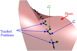
Sheet Tracking Algorithm]Block diagram of the sheet reconstruction algorithm. Picture (a) shows the propagation of the information around the main blocks. Block (A) is the initial position where the sheet tracking starts. Block (B1) corresponds to the iteration in the cross direction and bloc (C1) represents the iteration in the circumferential direction. For each iteration the position on the surface x^k+1 is stored and after triangulation is sent to the visualization module. (B2) and (C2) are the looping blocks with the switch and the buffer to save the previous position. 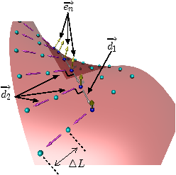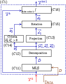The two loops are synchronized to do all the iterations in the d₂ directions for each in d₁. Picture (b) describes the circumferential iteration. (C11) is the MLS filtering and the decomposition is done in (C12). 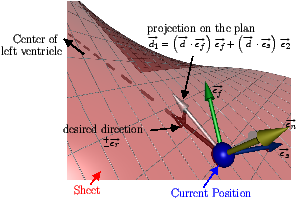There is the projection in (C13) and a positive sense is taken for e ₃ in (C14) to realize the rotation of d₁ in (C15). Then the integration step is performed in (C16). Picture (c) is the description of the cross section iteration. (B11) is the MLS regularization, (B12) is the decomposition into eigenvectors, the projection to get d₁ is realized in (B13) and the integration step is performed in (B14).

The first order Runge - Kutta method was used to reconstruct the sheet plane. The data were also filtered with the same MLS method that was used for the fibers. Since the MSL method filters more in the circumferential than in the cross sectional direction, some oscillations could still persist along this direction. Therefore, to compensate for this lack of regularization, a Gaussian filter was used on the surface in order to get a smooth visualization for the more noisy extremities (the midwall usually didn't need it).

2.4 Visualization of the Fiber and Sheet Tracking Results

The fibers were represented as tube-like surfaces with a radius of ≃ 400 μ m. Sheets defined as a set of parameterized points were triangulated creating meshed surfaces. The tubes and triangulated surfaces were displayed using the open source ray tracer POV-Ray (Persistence Of Vision Raytracer) (http://www.povray.org). We choose the software for the quality of the rendering which is by far better than the triangle based renderer. The POV-Ray scene description in a POV-Ray script language was generated by fiber and sheet tracking routines.

3 Results

3.1 Fiber Tracking

Reults of fiber tracking are presented and summarized in Figs. 8, 9 and 10. The visualization uses a color coding representation of the local fiber angle α. Clockwise rotation was encoded with a blue color and couterclockwise with a green color. The intensity of the coloration depends on the value of α. The dark blue and dark green represent larger angles for the epicardium and endocardium, respectively. The light blue in the midwall indicates fibers located in the axial plane. On each picture the color intensity is scaled to its maximum angle.

[] []

Fig. 8: [

Fiber Tracking result I]Figure (a) is the visualization of the fiber structure in the left ventricle. The visualization was created by using a cylindrical mesh of 1000 seed points throughout the entire volume. Clockwise to counterclockwise geometry of the fibers from the epicardium to endocardium can be seen. The nearest wall is the septum. Figure (b) is the display of the heart with the posterior wall on the bottom. Some differences can be seen in the angle intensity depending on the region.

[] []

Fig. 9: [

Fiber Tracking result II]Figure (a) represents a short section of the left ventricle which illustrates the smooth variation of the angle α and its sign inversion across the wall from epi- to endo-cardiac wall. Figure (b.) is the orientation of the fibers by sections around the left ventricle. For each section, the fibers are plotted closer to the endocardium. The smooth change of direction can be seen while the fiber bundle wraps around the endocardium.

[] []

Fig. 10: [

Fiber Tracking result III]Figure (a) is the helical visualization of the fibers from apex to base. The global homogeneity of the angle α can be seen. Figure (b) results of a fiber tracking close to the apex. The twist around it can be appreciated. It is worth noticing the smooth continuity of some bundle of fibers going down from the endocardium (green), pass the midwall (in light blue) and going up again (dark blue). The large variations between green and blue in the middle of the apex are due to the fast change of the clockwise to counterclockwise rotation. In the center, the comparison between clockwise and counterclockwise rotation is not accurate as the fibers become more aligned with the central axis of the left ventricle.

The fiber tracking was also performed for the entire heart. Figure 11 shows the fibers in the left and right ventricle. The helical rotation of the fibers can also be noticed in the right ventricle and the color encoding of the fiber is the same as the previous visualization.

Fig. 11: [

Fiber Tracking whole heart]Fiber tracking performed in the left and right ventricle. The closer part is the posterior wall of the right ventricle. The helical rotation can still be noticed in the right ventricle even though the smooth change of orientation across the wall is not as clear as that in the left ventricle. A continuity between left and right ventricle can be noticed in the posterial wall where the epicardial fibers of the left ventricle join smoothly to the right ventricle. However, the septal wall doesn't seem to be diretly linked to the right ventricle. In the basal region of the anterior wall of the right ventricle, the hole in the fibers is due to the link of the RV with the pulmonary artery.

Figure 12 is the results of the fiber tracking performed in the region of the anterior papillary muscle. Smaller fibers are drawn by seeding more precisely in the region of the papillary muscle. The color encodes the z component of the fiber. The green color encodes fiber with a large vertical orientation and the blue color orients a fiber with a more planar orientation.

Fig. 12: [

Fiber Tracking papillary muscle]Result of the fiber tracking in the papillary muscle. The small picture illustrates where the section is located in the heart geometry. The section shows the interio view of the anterior wall of the heart. The yellow part represents the region of the papillary muscle where the seeding was performed. The larger picture is a zoom on this region and shows the fiber geometry. The color encodes the z component of the fiber direction. The blue fibers have a planar orientation (mainly the fibers of the endocardium). The green fibers have a more vertical direction. The fiber orientation change completely in the papillary muscle where the fibers pass from a helical rotation (at the endocardium) to a clear vertical direction in the muscle.

3.2 Sheet Reconstruction

The surfaces of the sheet structures presented in Figs. 13, 14, 15 and 16 were constructed starting with seed points positioned in the midwall and grown in four directions (see Fig. 6(b))

[] []

Fig. 13: [

Sheet Tracking result I]Figure (a) shows a parameterized reconstructed surface of one sheet. The line traveling left from the closest corner corresponds to the epicardium. The structure is then going up circumferentialy. At the opposite end, the sheet goes down, following the fibers. The concave movement in the z coordinate is characteristic of a region close to the base of the left ventricle. The mesh shows the organized reconstruction of the surface. Figure (b) is the sheet surface and the corresponding fibers are visualized to understand their relationship. It can be noticed that the fibers lie completely on the surface. The color of the fiber is the visualization of the sense of rotation used previously. The color on the surface shows the third component of the fiber direction (red for a flat direction and blue for a large z component). The surface goes up clockwise with the fibers in the epicardial region, have a local maximum in the midwall where some circumferential fibers lie on it, and then goes down, twisting in the opposite direction with the fibers.

[] []

Fig. 14: [

Sheet Tracking result II]Figure (a) represents the sheets stacked crossing the ventricular wall. The directionality of each sheet going across the wall can be seen. The twist of the sheets is noticeable with a concave curvature in the transverse section of the heart wall. (The color of the sheet is only used to differentiate them, the endocardium is the red surface and the epicardium is shown by the mesh). This makes sense with the direction of the fibers on the region (going from clockwise to counterclockwise). The view of the sheet architecture in the lateral wall is shown in Figure (b). The global movement of twist across the wall is visible as well as the smooth variation of the normal orientation on different sheets depending on there z location. (The color here does not indicate information).

[] []

Fig. 15: [

Sheet Tracking result III]Figure (a) shows some large color coded sheets around the left ventricular positioned in the basal region. The color of the sheet encodes the z component of the fiber direction (the blue intensity is for a planar fiber and red for a fiber going up or down). Some noise can be seen in the epicardium. The color of the endocardium encodes the z component of the sheet normal. The green color indicates a large z component, meaning that the sheet is almost in the radial plane of the ventricle. At the opposite, the white transparent color indicates a normal directed more perpendicular to e _z, in these regions, sheets are less planar. The seeding of small sheets on the left ventricle is represented in Figure (b). The spatial variation of the orientation of these surfaces is shown. The color encoding on the surface is the same as in (a). Some regions can be differentiated where the cleavage planes fit well to the model crossing the wall and some other are far more vertical. The global structure is therefore complex. The color of the endocardium is the first and second component of the fiber. Thus, the rotation of the fiber structure around the endocardium can be seen.

Fig. 16: [

Sheet Tracking result IV]Seeding of sheets in the apex. Theses sheets smoothly join the epicardium to the endocardium. The color of the surface is encoding the third component of the fiber direction. In the region where the fibers are almost flat (red regions), the surface has very little twist and is almost planar. In the other case where the fibers have a large z component, the twist of the sheet is greater. The structure in the septal wall are not shown. This is because at this region the heart is linked with the right ventricle. The algorithm does not perform well due to the assumptions of how the surfaces cross the left ventricle which probably differ from surfaces embedded in the right ventricle.

4 Conclusion and Future Work

We presented a method for generation of high resolution and high quality visualization of fiber and laminar cardiac structures. In our implementation, the fibers were represented as shaded 3D tubes to improve the depth perception of the structure. It is well known from the literature that the fiber angles vary smoothly across the wall, and this work confirms that finding as seen in Fig. 9. However, we found that the generalization frequently used in the literature that the angle varies from +60^∘ to −60^∘ is just a rough approximation. The myocardium has a much more complex fiber structure especially close to the boundaries of the myocardial wall where the angles change directions very rapidly [5]. Using our approach, the apex of the heart was studied, and is presented in Fig. 10(b) and 16. Interestingly, the twist of the fiber bundles predicted by Torrent-Guasp et al. [48] was found as visualized in Fig. 10(b). The continuity between right and left ventricle joined by the posterior wall can also be seen with the view of both ventricles in Fig. 11. The structure of the sheet compares well with histological measurements from apex to base transmural sections [49],[9] (Fig. 14). The relationship between fiber directions and laminar structure is not obvious and our work helps to understand these relationships by providing high quality visualizations of both of these structures (Fig. 13(b) and 16). Fibers lie within the sheet surfaces, but the knowledge of fiber directions is not sufficient to create visualization of the cleavages planes. This implies that the surfaces need parameterizations which are not related to the fiber directions. The apex of the heart is an interesting region where the sheets have larger curvature due to the twist of the fibers. This rotation is especially visible in the lateral wall and contributes probably to the twisting movement of the apex. We found the process of fiber tracking sensitive to the noise but it is hard to characterize it as we are unsure in some cases whether the variation in fiber and sheet configuration is real or it is due to noise. An anisotropic filtering used in this work helps to regularize the process of tracking the fibers and sheets but introduces bias due to error of interpolation. Therefore, the following of the fiber over long distances may introduce large errors. In order to minimize these, we used first the Runge - Kutta method with an automatic error estimation that enabled the reduction of the errors in the numerical solution of the differential equations. Then, the anisotropic filtering was also performed to enable the reduction of the data errors. This regularization was performed for each position given by the local direction of the fiber. As the fiber direction is obtained based on the largest eigenvector only, the noise is not a significant problem. But it is more significant for the determination of the sheet structure which is obtained based on the second and third eigenvector which are smaller and noisier. The first eigenvector has an amplitude λ₁ and is significantly greater than the two others which make it easy to distinguish the e₁ from the other two eigenvectors. For e₂ and e₃, however, the respective eigenvalues are far more close to each other[36]. With this in mind, taking λ₂>λ₃, a small amount of noise can easily invert the relation and therefore invert e_n and e_s. This implies that the mathematical problem of finding the plane is ill-posed. A criteria to verify the correct interpretation of the two last eigenvectors could be developed to avoid this misclassification by having an a priori constraint on the orientation of the sheet normal. Another problem is the noise level for e₂ and e₃. The two smallest eigenvectors have lower amplitudes than the first component and therefore are subject to stronger noise effects. We can especially appreciate this effect close to boundaries of the walls, where some results of the surfaces oscillate (Figure. 14(a), 15(a)). A filter similar to the moving least square that we used for fiber tracking can also help for sheet tracking to reduce these artifacts. The last problem that we would like to point out is the structure of the sheet itself. We assume that the sheet goes mainly across the wall. If this direction is not the real direction of the sheet, our projected vector does not control well the directionality of the tracking, and it can lead to an arbitrary direction of construction with amplitude that can approach zero. This problem appears specifically in the middle part of the anterior wall where the normal directions of the sheets are almost transverse to the wall. In order to resolve this problem another parameterized direction may be used in this region ([37], [16]). The noise characterization of the sheet surfaces is therefore a complex problem. And as the precise structure of this is not well known, conclusions concerning surface oscillations based on the anatomical or noisy origin of those cannot be taken. The sheet tracking algorithm was performed with the same regularized field that was used for the fiber tracking. This enabled the tracked fibers to lie exactly inside the surface. However another MLS regularization could also be implemented to filter more in the spanned direction of the sheet than in the normal direction. A differentiation between the two smallest eigenvectors should then be taken. For this work, there are several avenues of continuation . One interesting avenue is to compare the detected planes with the directions of the major principal strains of cardiac deformation (see for example Fig. 10 in [3]). It is expected that the largest strains found in the analysis of the deformation should align with the cleavage surfaces. Another way of using our method is to perform an analysis of the fiber direction distribution and laminar structure for the case of the failing heart where remodeling can be studied as a function of changes in fiber and sheet structures. The presented method can also be used to study the effect of surgical procedures on the fiber and sheet structures in the myocardium using some animal model [23]. For this application, the visualization aspect of our work would be very important. Other regions of the heart could also be studied. A more detailed study of the structure of the right ventricle could be performed (Fig. 11). The regions of the papillary muscles could also be studied. Since the fiber clearly change orientation (Fig. 12) the correlation between fiber structure and physiological characteristics would be of interest. Some limitations still remain. Some of them are linked to the choice of POV-Ray software used for visualization. The visualization is performed by ray tracing and because of that it is very slow compared to other libraries such as OpenGL. Therefore, at the current stage of our research, interactive viewing of the results of the fiber and sheet tracking is not possible. Making our visualization interactive will be the next step that we will take. Finally, we plan to validate the hypothesis of a cardiac band [48, 50, 51, 52, 53] where it is postulated that the four chamber heart is built from a single continuous band of muscle.

Acknowledgments

This work was supported by NIH Grant R01 EB000121 and U.S. Department of Energy (DOE) under contract DE-AC02-05CH11231. The authors acknowledge Drs. Patrick A. Helm and Raimond L. Winslow at the Center for Cardiovascular Bioinformatics and Modeling and Dr. Elliot McVeigh at the National Institute of Health for providing the data. The Data may be accessed on the internet at www.ccbm.jhu.edu .

References

[1]: Susumu Mori and Peter B. Barker. Diffusion magnetic resonance imaging : Its principle and applications. The Anatomical Record, 257(3):102–109, 1999.
[2]: Guus Berenschot. Visualization of diffusion Tensor Imaging. PhD thesis, Eindhoven University of Technology, 2003.
[3]: Burkhard Wunsche. The visualization and measurement of left ventricular deformation. In Proceedings of the First Asia-Pacific Bioinformatics Conference on Bioinformatics, pages 119–128. Australian Computer Society, Inc., 2003.
[4]: Jane Sands Robb and Robert Cumming Robb. The normal heart, anatomy and physiology of the structural units. American Heart Journal, 23(4):455–467, April 1942.
[5]: Daniel D. Streeter, Henry M. Spotnitz, Dali P. Patel, John Ross, and Edmund H. Sonnenblick. Fiber orientation in the canine left ventricle during diastole and systole. Circulation Research, 24(3):339–347, March 1969.
[6]: Henry M. Spotnitz. Macro design, structure, and mechanics of the left ventricle. The Journal of Thoracic and Cardiovascuar Surgery, 119(5):1053–1077, May 2000.
[7]: T. Arts, K. D. Costa, J. W. Covell, and A. D. McCulloch. Relating myocardial laminar architecture to shear strain and muscle fiber orientation. American Journal of Physiology. Heart and Circulatory Physiology, 280(5):2222–2229, May 2001.
[8]: Kevin D. Costa, Yasuo Takayama, Andrew D. McCulloch, and James W. Covell. Laminar fiber architecture and three-dimensional systolic mechanics in canine ventricular myocardium. American Journal of Physiology. Heart and Circulatory Physiology, 276(2):595–607, February 1999.
[9]: Peter J. Hunter, Bruce H. Smaill, Poul Nielsen, and Ian J. Le Grice. Computational Biology of the Heart, chapter 6. A Mathematical Model of Cardiac Anatomy. John Wiley, April 1996.
[10]: Robert H. Hoyt, Mark L. Cohen, and Jeffrey E. Saffitz. Distribution and three-dimensional structure of intercellular junctions in canine myocardium. Circulation Research, 64(3):563–574, March 1989.
[11]: Karl T. Weber, Yao Sun, Suresh C. Tyagi, and Jack P. M. Cleutjens. Collagen network of the myocardium: Function, structural remodeling and regulatory mechanisms. Journal of Molecular and Cellular Cardiology, 26(3):279–292, March 1994.
[12]: Paul W.M. Fedak, Subodh Verma, Richard D. Weisel, and Ren-Ke Li. Cardiac remodeling and failure from molecules to man (Part II). Cardiovascular Pathology, 14(3):109–19, March 2005.
[13]: J Ohayon and R S Chadwick. Effects of collagen microstructure on the mechanics of the left ventricle. Biophysical Journal, 54(6):1077–1088, December 1988.
[14]: E. W. Hsu, A. L. Muzikant, S. A. Matulevicius, R. C. Penland, and C. S. Henriquez. Magnetic resonance myocardial fiber-orientation mapping with direct histological correlation. American Journal of Physiology. Heart and Circulatory Physiology, 274(5):1627–1634, May 1998.
[15]: TF Robinson, MA Geraci, EH Sonnenblick, and SM Factor. Coiled perimysial fibers of papillary muscle in rat heart: Morphology, distribution, and changes in configuration. Circulation Research, 63(3):577–592, September 1988.
[16]: Katherine B. Harrington, Filiberto Rodriguez, Allen Cheng, Frank Langer, Hiroshi Ashikaga abd George T. Daughters, John C. Criscione, Neil B. Ingels, and D. Craig Miller. Direct measurement of transmural laminar architecture in the anterolateral wall of the ovine left ventricle: New implications for wall thickening mechanics. American Journal of Physiology. Heart and Circulatory Physiology, 288(3):1324–30, March 2005.
[17]: Alexander I. Veress, Grant T. Gullberg, and Jeffrey A. Weiss. Measurement of strain in the left ventricle during diastole with cine-MRI and deformable image registration. Journal of Biomechanical Engineering, 127(7):1195–1207, December 2005.
[18]: Hiroshi Ashikaga, John C. Criscione, Jeffrey H. Omens, James W. Covell, and Jr. Neil B. Ingels. Transmural left ventricular mechanics underlying torsional recoil during relaxation. American Journal of Physiology. Heart and Circulatory Physiology, 286(2):640–647, October 2004.
[19]: Socrates Dokos, Bruce H. Smaill, Alistair A. Young, and Ian J. LeGrice. Shear properties of passive ventricular myocardium. American Journal of Physiology. Heart and Circulatory Physiology, 283(6):2650–2659, December 2002.
[20]: Yasuo Takayama, Kevin D. Costa, and James W. Covell. Contribution of laminar myofiber architecture to load-dependent changes in mechanics of LV myocardium. American Journal of Physiology. Heart and Circulatory Physiology, 282(4):1510–1520, April 2002.
[21]: Katarina Kindberg. Connection between strain in cardiac coordinates and strain in fiber coordinate. Technical report, Department of Biomedical Engineering, Linkopings Universitet, Sweden, July 2005.
[22]: Patrick A. Helm, Laurent Younes, Mirza F. Beg, Daniel B. Ennis, Christophe Leclercq, Owen P. Faris, Elliot Mc Veigh, David Kass, Michel I. Miller, and Raimond Winslow. Evidence of structural remodeling in the dyssynchronous failing heart. Circulation Research, 98(1):125–132, January 2006.
[23]: Joseph C. Walker, Julius M. Guccione, Yi Jiang, Peng Zhang, Arthur W. Wallace, Edward Hsu, and Mark B. Ratcliffe. Helical myofiber orientation after myocardial infarction and left ventricular surgical restoration in sheep. Journal of Thoracic and Cardiovascular Surgery, 129(2):382–390, February 2005.
[24]: Scott D. Zimmerman, John Criscione, and James W. Covell. Remodeling in myocardium adjacent to an infarction in the pig left ventricle. American Journal of Physiology. Heart and Circulatory Physiology, 287(6):2697–704, December 2004.
[25]: Junjie Chen, Sheng-Kwei Song, Wei Liu, Mark McLean, J. Stacy Allen, Jie Tan, Samuel A. Wickline, and Xin Yu. Remodeling of cardiac fiber structure after infarction in rats quantified with diffusion tensor MRI. American Journal of Physiology. Heart and Circulatory Physiology, 285(3):946–954, May 2003.
[26]: Marc A. Pfeffer and Eugene Braunwald. Ventricular remodeling after myocardial infarction. experimental observations and clinical implications. Circulation, 81(4):1161–1172, April 1990.
[27]: Paul W.M. Fedak, Subodh Verma, Richard D. Weisel, and Ren-Ke Li. Cardiac remodeling and failure from molecules to man (Part I). Cardiovascular Pathology, 14(1):1–11, January 2005.
[28]: H.C. Torrey. Bloch equations with diffusion terms. Physical Review, 103(3):563–565, November 1956.
[29]: Oliver Natt and Jens Frahm. In vivo magnetic resonance imaging: Insights into structure and function of the central nervous system. Measurement Science and Technology, 16:R17–R36, February 2005.
[30]: Evren Ozarslan and Thomas H. Mareci. Generalized diffusion tensor imaging and analytical relationships between diffusion tensor imaging and high angular resolution diffusion imaging. Magnetic Resonance in Medicine, 50(5):955–965, November 2003.
[31]: Denis Le Bihan, Jean-François Mangin, Cyril Poupon, Chris A. Clark, Sabina Pappata, Nicolas Molko, and Hughes Chabriat. Diffusion tensor imaging: Concepts and applications. Journal of Magnetic Resonance Imaging, 13(4):534–546, April 2001.
[32]: Denis Le Bihan. Looking into the functional architecture of the brain with diffusion MRI. Nature Reviews. Neuroscience, 4(6):459–80, June 2003.
[33]: Cyril Poupon. Détection des faisceaux de fibres de la substance blanche pour l'étude de la connectivité anatomique cérébrale. PhD thesis, Ecole Nationale Superieure des Telecommunications de Paris, Paris, France, 1999.
[34]: Susumu Mori and Peter C. M. van Zijl. Fiber tracking: principles and strategies - a technical review. Nuclear Magnetic Resonance in Biomedicine, 15(7-8):468–80, November-December 2002.
[35]: David F. Scollan, Alex Holmes, Raimond Winslow, and John Forder. Histological validation of myocardial microstructure obtained from diffusion tensor magnetic resonance imaging. American Journal of Physiology. Heart and Circulatory Physiology, 275(6):2308–2318, December 1998.
[36]: David Scollan. Reconstructing the Heart: Development and Application of Biophysically-Based Electrical Models of Propagation in Ventricular Myocardium Reconstructed from Diffusion Tensor MRI. PhD thesis, Johns Hopkins University, Baltimore, Maryland, 2002.
[37]: Patrick Helm, Mirza Faisal Beg, Michael I.Miller, and Raimond L.Winslow. Mesuring and mapping cardiac fiber and laminar architecture using diffusion tensor MR imaging. Annals of the New York Academy of Sciences, 1047:296–307, June 2005.
[38]: Leonid Zhukov and Alan H. Barr. Heart-muscle fiber reconstruction from diffusion tensor MRI. IEEE , Proceedings of the 14th IEEE Visualization, page 79, October 2003.
[39]: Peter J. Hunter, Andrew J. Pullan, and Bruce H. Smaill. Annual Review of Biomedical Engineering, volume 5, chapter 6. Modeling Total Heart Function. Annual Reviews, 2003.
[40]: Tim H.J.M. Peeters, Anna Vilanova, Gustav J. Strijkers, and Bart M. ter Haar Romeny. Visualization of the fibrous structure of the heart. IEEE Visualization 2006, 2006. Submitted.
[41]: Marcel Jackowski, Zakir Sahul, Maolin Qiu, Lawrence Staib, and Albert J. Sinusas. Reconstruction of myocardial fiber sheets using diffusion tensor imaging. Journal of Cardiovascular Magnetic Resonance, 8:16–17, January 2006. Abstract.
[42]: David Weinstein, Gordon Kindlmann, and Eric Lundberg. Tensorlines: Advection-diffusion based propagation through diffusion tensor fields. IEEE , Proceedings of the conference on Visualization, pages 249–254, 1999.
[43]: Leonid Zhukov and Alan H. Barr. Oriented tensor reconstruction: tracing neural pathways from diffusion tensor mri. IEEE , Proceedings of the Conference on Visualization '02, pages 387–394, October 2002.
[44]: Anders Brun Mats Bjornemo. White Matter Fiber Tracking using Diffusion Tensor MRI. PhD thesis, Linkoping University, Sweden, 2002.
[45]: E. Haier, S. P. Norsett, and G. Wanner. Solving Ordinary Differential Equations I, Nonstiff Problems. Springer, 2000.
[46]: O. Coulon, D. C. Alexander, and S. R. Arridge. Tensor field regularisation for DT-MR images. In British Conference on Medical Image Understanding and Analysis, Birmingham, United-Kingdom, 2001.
[47]: Xavier Pennec, Pierre Fillard, and Nicholas Ayache. A Riemannian framework for tensor computing. International Journal of Computer Vision, 66(1):41–66, January 2006.
[48]: Francisco Torrent-Guasp, Mladen J. Kocicab, Antonio F. Cornoc, Masashi Komedad, Francesc Carreras-Costae, A. Flotatsf, Juan Cosin-Aguillarg, and Han Wenh. Towards new understanding of the heart structure and function. European Journal of Cardio-Thoracic Surgery, 27(2):191–201, February 2005.
[49]: I. Legrice, P. Hunter, A. Young, and B. Smaill. The architecture of the heart: a data-based model. Royal Society of London Philosophical Transactions Series A, 359:1217, June 2001.
[50]: Francisco Torrent-Guasp, Mladen J. Kocicab, Antonio Cornoc, Masashi Komedad, James Coxe, A. Flotatsf, Manel Ballester-Rodesg, and Francesc Carreras-Costah. Systolic ventricular filling. European Journal of Cardio-Thoracic Surgery, 25(3):376–386, March 2004.
[51]: Ludwig K. von Segesser. The myocardial band: Fiction or fact? European Journal of Cardio-Thoracic Surgery, 27(2):181–182, February 2005.
[52]: Gerald D. Buckberg. Architecture must document functional evidence to explain the living rhythm. European Journal of Cardio-Thoracic Surgery, 27(2):202–209, February 2005.
[53]: Donald N. Ross. The morphology of the pulmonary root in relation to the human heart. The Annals of Thoracic Surgery, 72(3):976, September 2001.

This document was translated from L^AT_EX by H^EV^EA.